Getting started#

While there are a lot of complicated components to SkellySim, the basic workflow is easy.

Generate a configuration file

$ python gen_config.py skelly_config.toml
Generate precompute data

$ skelly_precompute skelly_config.toml
Run the simulation. Recommended in an sbatch script. See example submission script

$ mpirun skelly_sim --config-file=skelly_config.toml
Visualize or post-process

Example simulation full workflow#

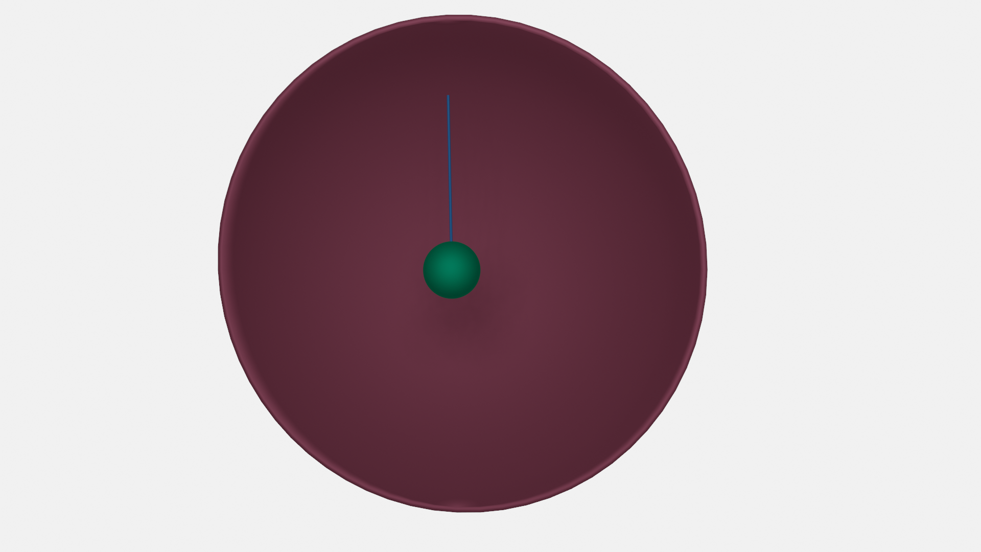
The following example is from our github. It represents a fairly minimal system which has a Fiber attached to a Body and a Periphery. The Body experiences a constant upward force, while the Fiber attaches and hinges to the Periphery when it gets close to it. For more details about the actual configuration generation process, you should check out generate a configuration file. If you’re using singularity, which we recommend to start with, note you’ll have to prefix all your commands as noted in the Installation page. Now, before we get into how to generate images, let’s show what this initial condition looks like

Download the example and put in a clean directory.

% ls
gen_config.py
% ./gen_config.py
Using default toml file for output: 'skelly_config.toml'. Provide an alternative filename argument to this script to use that instead.
% ls
gen_config.py skelly_config.toml

The config generation scripts we provide all default to making a ‘skelly_config.toml’ file, though this naming isn’t necessary. Your script can name the file whatever it likes, though using this default is nice since most scripts look for it. It’s also worth taking a look at the output just to see what’s inside, though there isn’t really much reason to peer into them unless you want to make a quick change to see what a parameter does.

The next step is to generate some precompute data which is used throughout the simulations (quadrature weights and matrix inversions). Use the skelly_precompute utility to do this. If you’re using a virtual environment or conda for the python portion, make sure to activate that environment first. Note that this can take some time, especially if your Periphery has a lot of nodes.

% skelly_precompute skelly_config.toml
{'nucleation_type': 'auto', 'n_nucleation_sites': 50, 'position': [0.0, 0.0, 0.0], 'orientation': [0.0, 0.0, 0.0, 1.0], 'shape': 'sphere', 'radius': 0.5, 'n_nodes': 400, 'precompute_file': 'body_precompute.npz', 'external_force': [0.0, 0.0, 0.5]}
Building Quadrature Weights
Finished building Quadrature Weights
Building Quadrature Weights
Finished building Quadrature Weights
Creating periphery object
Finished creating periphery object
Finished periphery init.
% ls
body_precompute.npz  gen_config.py  periphery_precompute.npz  skelly_config.toml

Now we have all our configuration and precompute data and are ready to run a simulation. Since this is a very basic simulation, there is no need to use mpirun, which will likely hinder more than help performance. When simulating thousands of fibers or giant Peripheries, mpirun becomes necessary. You may see some warnings about OpenMP from Kokkos. You can ignore the warning or do as it recommends. It may or may not help performance.

Run the simulation as follows. Then maybe go get a cup of coffee, as it should take a few minutes.

% skelly_sim
[2022-03-28 16:04:06.968] [SkellySim] [info] ****** SkellySim 0.9.3 (a5a5baae) ******
[2022-03-28 16:04:06.971] [SkellySim] [info] Preprocessing config file
[2022-03-28 16:04:06.972] [SkellySim] [info] Initializing FiberContainer
[2022-03-28 16:04:08.645] [SkellySim] [info] Reading in 1 fibers.
[2022-03-28 16:04:10.706] [SkellySim] [info] Loading raw precomputation data from file periphery_precompute.npz for periphery into rank 0
[2022-03-28 16:04:11.032] [SkellySim] [info] Done initializing base periphery
[2022-03-28 16:04:14.660] [SkellySim] [info] Reading in 1 bodies
[2022-03-28 16:04:14.737] [SkellySim] [info] Body 0: [ 0, 0, 0 ]
[2022-03-28 16:04:15.691] [SkellySim] [info] Solver converged with parameters: iters 7, time 0.3280859529040754, achieved tolerance 4.6319964036583045e-11
[2022-03-28 16:04:15.731] [SkellySim] [info] Residual: 1.824888062028897e-07
[2022-03-28 16:04:15.731] [SkellySim] [info] Accepting timestep and advancing time
[2022-03-28 16:04:15.732] [SkellySim] [info] System time, dt, fiber_error: 0.1, 0.1, 2.0501852452392555e-06
etc...
% ls
body_precompute.npz  gen_config.py  periphery_precompute.npz  skelly_config.toml  skelly_sim.out

We now have one more file ‘skelly_sim.out’. This is the trajectory information. This contains all solution information at all output times in a binary nested dictionary format msgpack (which is similar to json).

To visualize this, you should be able to open it with our provided blend file (just make sure to put the skelly_blend.py script with it in the same directory. This process isn’t standardized yet unfortunately). By default these are both in the source scripts directory. This doesn’t need the Singularity container or any install at all. Just the ‘skelly.blend’ and ‘skelly_blend.py’ files. The first time the script is run it should bootstrap itself to work with Blender’s packaged Python.

% blender  ~/projects/codes/SkellySim/scripts/skelly.blend -y

Will open Blender, find the simulation, and set up a scene and animation for it. Just make sure to run it from the simulation directory. Also, note the ‘-y’ option, which allows Blender to execute scripts, which our setup depends on. Otherwise you’ll have to click a dialog menu.

If you’d like to animate it, you can use the standard gui facilities, or you can run Blender in batch mode.

% blender  ~/projects/codes/SkellySim/scripts/skelly.blend -y -b -o movie -F AVIRAW -a

will generate a very very large AVI file in your simulation directory (likely named movie0000-0199.avi) in this specific case. If you have a working ffmpeg install (or another utility of your choice), you can compress this by a few orders of magnitude without real loss of quality.

% ffmpeg -y -r 60 -i movie0000-0199.avi -vcodec libx264 -crf 10 -r 60 movie.mp4

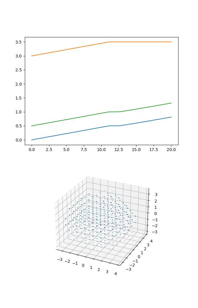
Now we probably want to do some analysis. The following code loads in a trajectory and plots vs time the ‘z’ coordinates of the body, the fiber plus end, and the fiber minus end in the body_fiber_periphery_constant_body_force example. It also generates a 3d quiver plot of the velocity field at the 11th time frame of the velocity field. The full code is in the examples/analysis_example.py script.

import numpy as np
import matplotlib
matplotlib.use('TKAgg')
import matplotlib.pyplot as plt

from skelly_sim.reader import TrajectoryReader, Listener, Request

traj = TrajectoryReader('skelly_config.toml')
shell_radius = traj.config_data['periphery']['radius']
body_radius = traj.config_data['bodies'][0]['radius']

body_pos = np.empty(shape=(len(traj), 3)) # COM body position in time
plus_pos = np.empty(shape=(len(traj), 3)) # fiber plus end in time
minus_pos = np.empty(shape=(len(traj), 3)) # fiber minus end in time

for i in range(len(traj)):
    traj.load_frame(i)
    body_pos[i, :] = traj['bodies'][0]['position_']
    minus_pos[i, :] = traj['fibers'][0]['x_'][0, :]
    plus_pos[i, :] = traj['fibers'][0]['x_'][-1, :]

print("system keys: " + str(list(traj.keys())))
print("fiber keys: " + str(list(traj['fibers'][0].keys())))
print("body keys: " + str(list(traj['bodies'][0].keys())))
print("shell keys: " + str(list(traj['shell'].keys())))

ax1 = plt.subplot(1, 2, 2)
ax1.plot(traj.times, body_pos[:, 2], traj.times, plus_pos[:,2], traj.times, minus_pos[:,2])

# Fire up SkellySim in "listener" mode
listener = Listener(binary='skelly_sim_release')

# All analysis requests are done via a "Request" object
req = Request()

# specify frame number to evaluate and evaluator (CPU, GPU, FMM)
req.frame_no = 11
req.evaluator = "GPU"

# Request velocity field
tmp = np.linspace(-shell_radius, shell_radius, 20)
xm, ym, zm = np.meshgrid(tmp, tmp, tmp)
xcube = np.array((xm.ravel(), ym.ravel(), zm.ravel())).T

# Filter out points outside periphery and inside body
relpoints = np.where((np.linalg.norm(xcube - body_pos[11,:], axis=1) > body_radius) &
(np.linalg.norm(xcube, axis=1) < shell_radius))
req.velocity_field.x = xcube[relpoints]

# Make our request to SkellySim! Might take a second...
res = listener.request(req)

x = req.velocity_field.x
v = res['velocity_field']

ax2 = plt.subplot(1, 2, 2, projection="3d")
ax2.quiver(x[:, 0], x[:, 1], x[:, 2], v[:, 0], v[:, 1], v[:, 2])

plt.show()

% python ../analysis_example.py
Loading trajectory index.
Loading trajectory index.
Stale trajectory index file. Rebuilding.
system keys: ['time', 'dt', 'rng_state', 'fibers', 'bodies', 'shell']
fiber keys: ['n_nodes_', 'length_', 'length_prev_', 'bending_rigidity_', 'penalty_param_', 'force_scale_', 'beta_tstep_', 'epsilon_', 'binding_site_', 'tension_', 'x_']
body keys: ['radius_', 'position_', 'orientation_', 'solution_vec_']
shell keys: ['solution_vec_']

SkellySim 0.9.12 documentation

Getting started

Contents

Getting started#

Example simulation full workflow#