What does a typical (generalized) eigenfunction of the Laplacian in the unbounded domain R², ie 2D free space, look like? If the eigenvalue is k², then we are considering a random solution to the Helmholtz equation with wavenumber k. Say we choose unit wavenumber k=1 then the complex plane wave e^in.x, with n is a unit direction vector, is an eigenfunction, but is not typical. A typical sample from the eigenspace with eigenvalue 1 can be constructed by a superposition of such waves traveling in all directions, with random complex phases. In other words, it is the 2D Fourier transform of Gaussian white noise restricted to the unit circle S¹. Berry first proposed this as a model for quantum eigenfunctions of systems whose classical dynamics is chaotic, in the '70s.

Below we show some pictures, investigations, and the version on the surface of a sphere; but first some code.

Codes

Here is MATLAB code to generate samples from the random plane wave ensemble, for the above monochromatic case (α=1 in Sarnak's notation), and for the case of integrating over all wavenumbers [0,1] (α=0 or Fubini-Study in Sarnak's notation):

• 2D code using FINUFFT: rpw2dfinufft.m. See the MATLAB help for documentation and example usage. It is O(N^2 log N) for a grid with N points on a side, and gives by default around 8 digits uniform accuracy over the output domain.

Here are my old codes (OBSOLETE):

• 2D code (need CMCL's NUFFT): rpw2dnufft.m.

• 2D code: rpw2dsample.m which needs codes circle_blobs.m and src.m. See the MATLAB help for documentation and example usage. The code is spectrally accurate (with default parameter e=5 it has absolute errors of order 3e-4), and uses my own nonuniform FFT implementation by resampling onto a uniform square grid of size 4N on a side. In 2014 I returned to this and realized that the NUFFT should only need size 2N on a side, so decided to use an existing NUFFT implementation.

• For larger computations the windowed NUFFT becomes a RAM-hog and crude slow-FT summation wins out if you have CPU cycles to burn. Here's a code for that: naiverpw.m. It was used for the 2000-wavelength boxes below in 2009; now in 2023 the above code rpw2dfinufft can do the same job on a laptop in a few seconds.

Pictures and Investigations

Random plane waves was one of the topics addressed at the AIM Workshop on Topological complexity of random sets (Aug 2009). Here is my contribution to the workshop, and some data generated there is below.

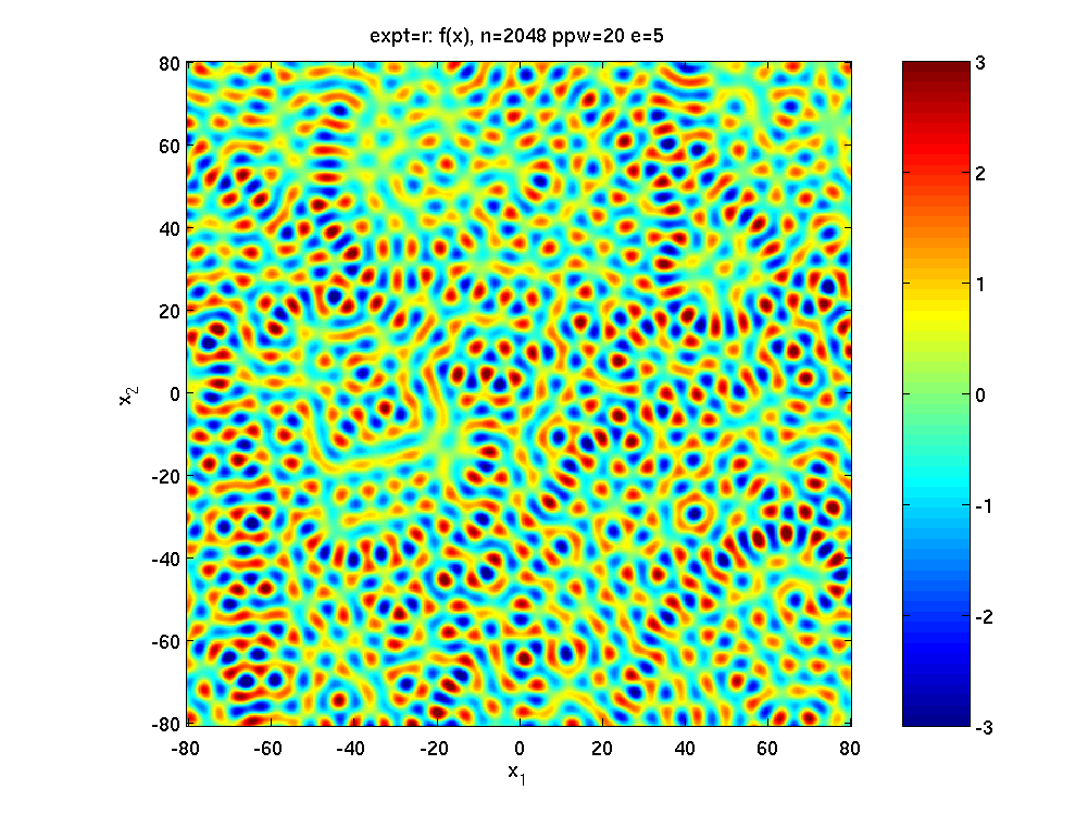
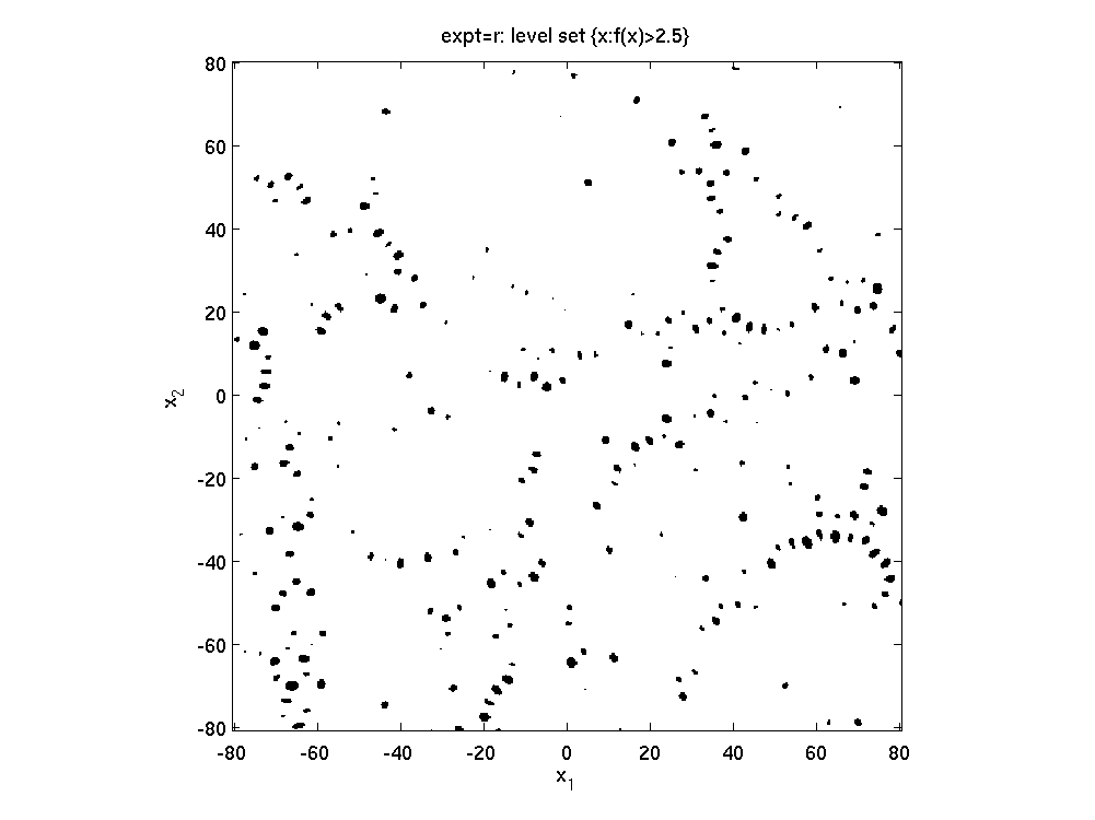
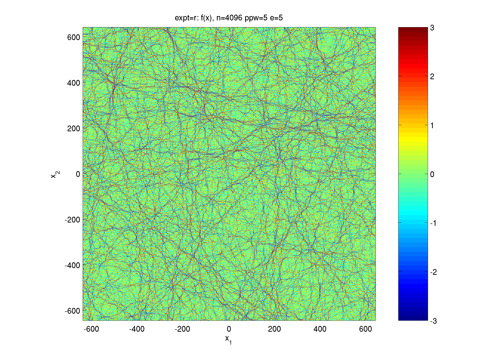
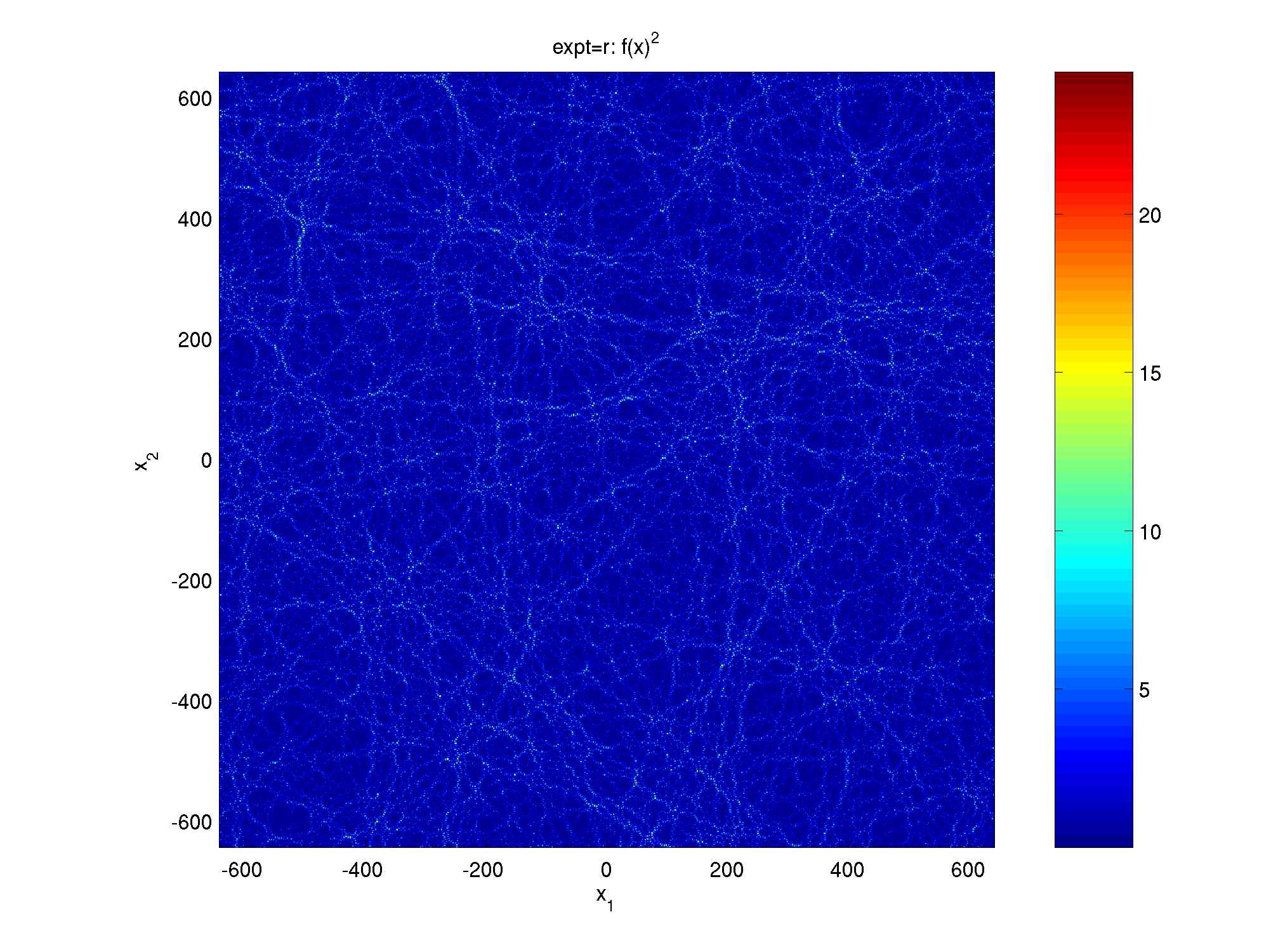
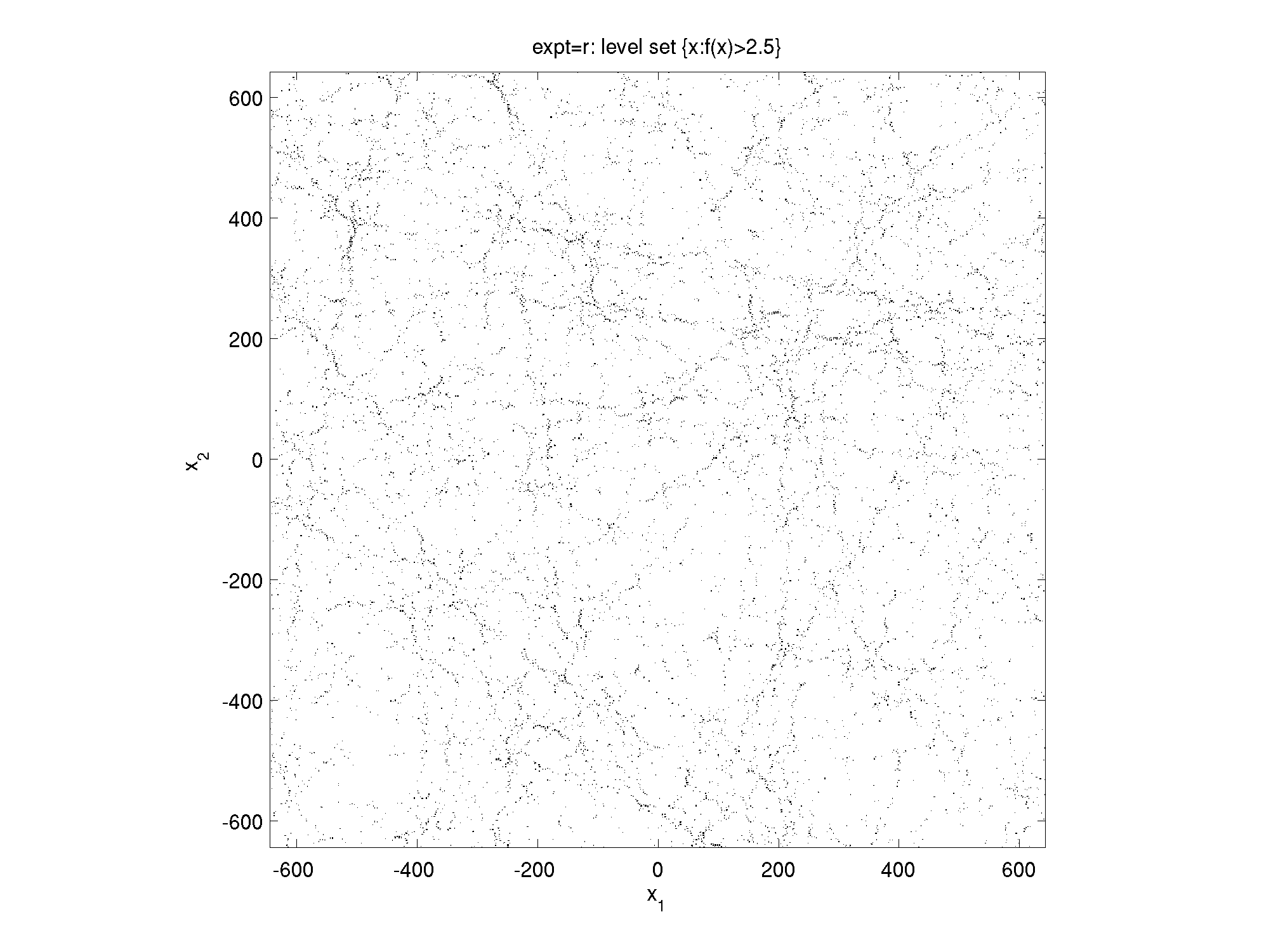
Here are some pictures of samples of random plane waves, showing the real part, chosen with mean-square value 1, computed with the code linked below. Click on each to magnify:

	color plot	squared	extreme value set (|f|>2.5)
25 wavelengths box
200 wavelengths box

One might study the local box-counting (Kolmogorov) fractal dimension of the extreme-value sets via the slope of the log-log plot of the number of boxes vs box size. Here is such a plot (different curves are for the different extreme value cut-offs), compared to the same for a spatially-uncorrelated model. They are similar but the stringiness of the level-set shows up as a slight slope in the region before the asymptotic slope of 2 is reached.

Some movies generated at the workshop:

• 200 wavelengths box with varying extreme value cut-off (6MB, black is above, white below, the value shown at bottom right).
• 2000 wavelength box with varying extreme value cut-off (3MB, black is below, white above, the value shown at top right), downsampled from 7000x7000 data below.
• color version (3MB) of the above.
• Worms movie (4MB) of slowly changing spectral measure from the whole disk, through an annulus, to a very thin annulus. Notice how the correlation length-scale grows.
• Mark Dennis' worms movie (4MB) of the same thing, instead using radially-sliding point-masses as spectral measure.

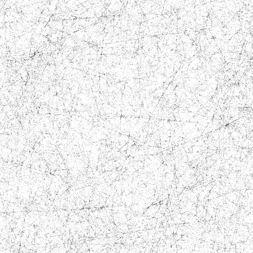
Here is a super-large plane-wave sample, showing the extreme-value set downsampled from 7000x7000 pixels, 2000 wavelengths across (click to magnify):

extreme-value set |f|>3.0

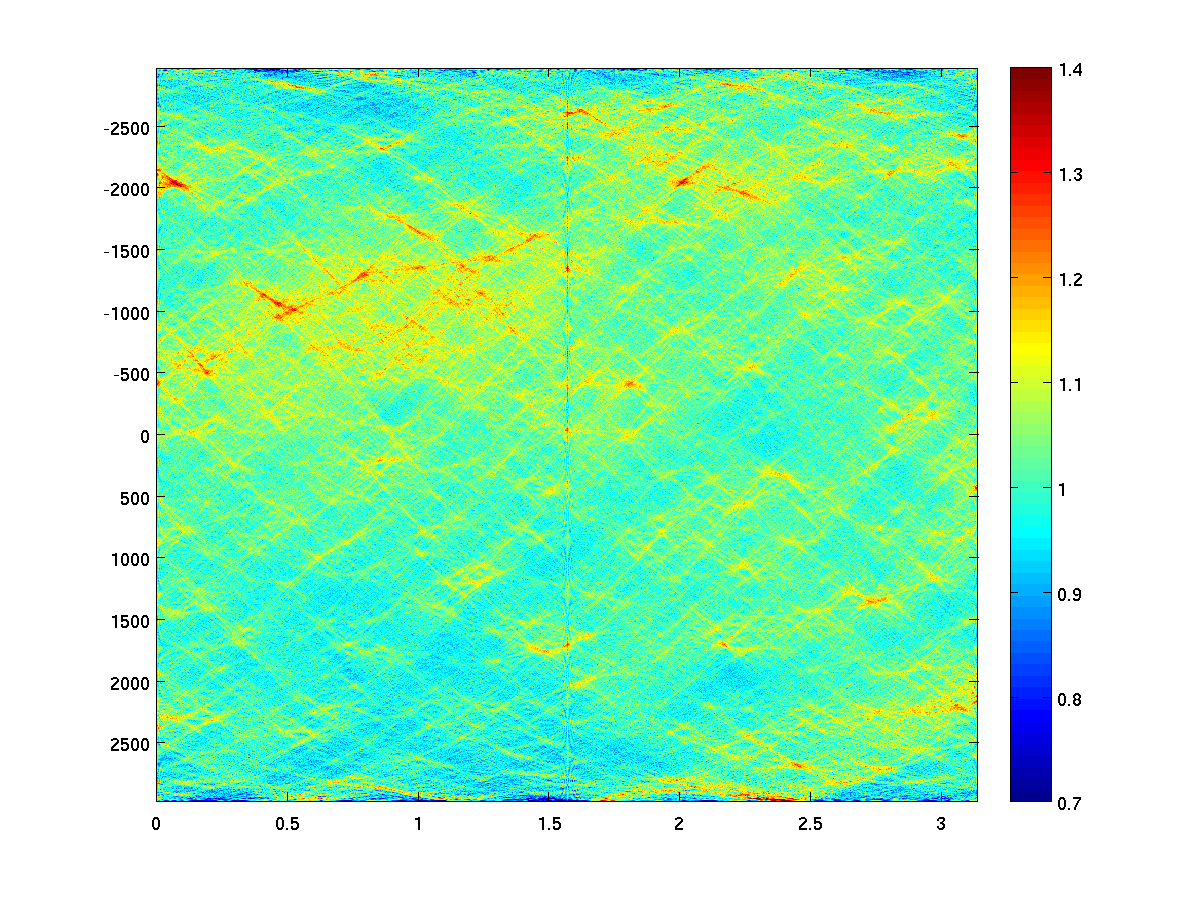
mean Radon projection of (bottom-left quarter of) f2

Notice how the Radon projection seems to have isolated bright spots (or bowties), as you'd expect for intense lines in coordinate space. It is an open problem how to prove something statistical which quantifies the `stringiness' visible to the eye in the above pictures and movies. One question is why the Radon, or Gaussian beam, basis, leads to apparent sparsity of coefficients.

Some references (also see AIM contribution above):

• "Properties of random superpositions of plane waves", P. O'Connor, J. Gehlen, E. J. Heller, Phys. Rev. Lett. 58, 1296-1299 (1987). This paper was how I first learned about this, showing that when the wavenumbers are allowed to vary in magnitude, the stringiness disappears.
• Terence Tao's notes on Tomas-Stein theorems on restrictions of the Fourier transform to the sphere. This seems not to be relevant since the functions do not live in L^p spaces.
• "Filament structure of random waves", Melissa Tacy, Nonlinearity 36(3), 1547-1570 (2023). In this recent open-access article, Tacy (with whom I have collaborated on other work) applies microlocal analysis estimates to rule out the possibility of logarithmic concentration along long lines, but shows that the filament structure may be a configuration-space echo of phase-space concentration. It is also an excellent review of the mathematical literature on this topic.

Random Spherical Harmonics

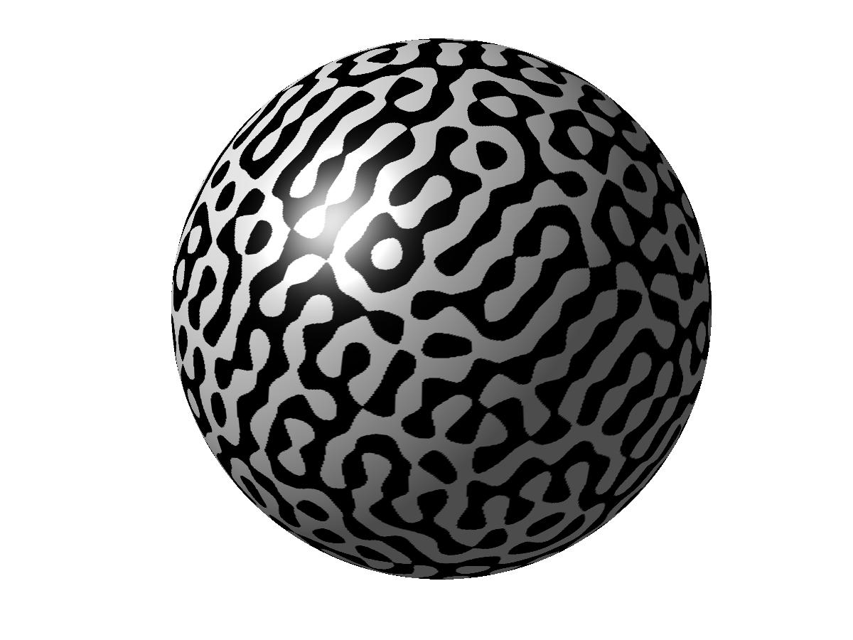
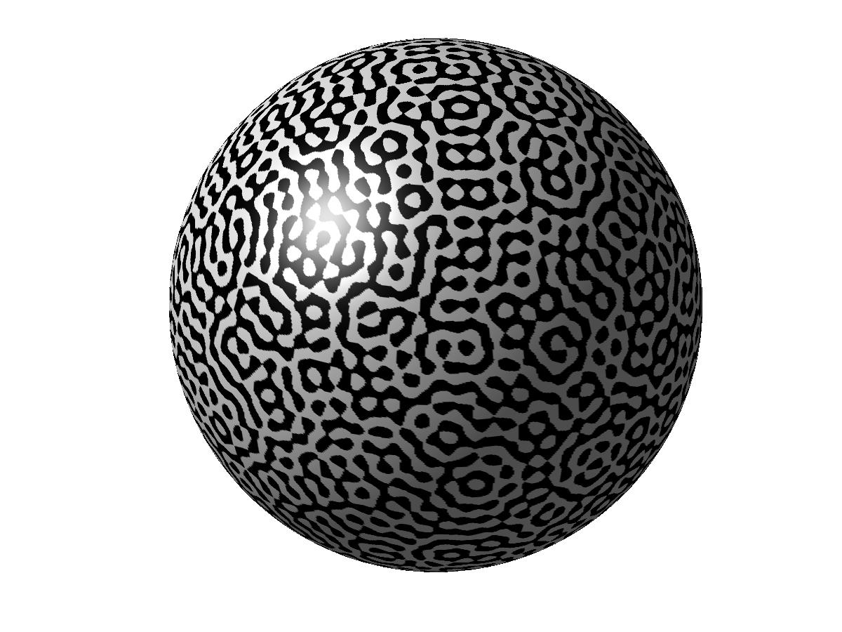
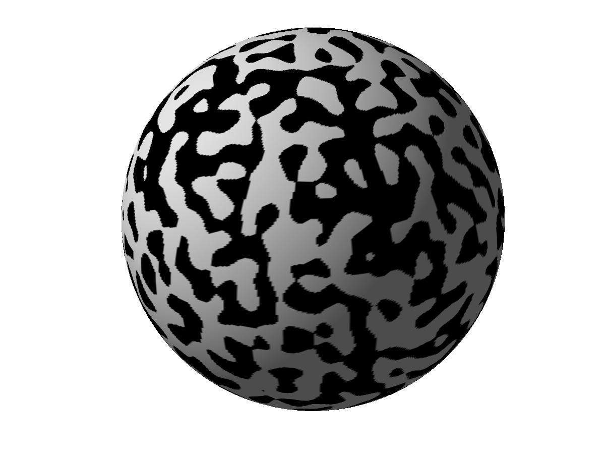
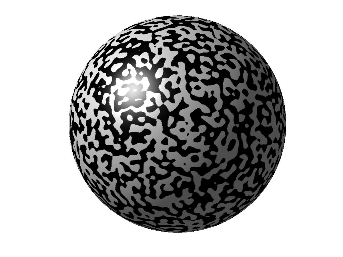
How about random plane waves on a sphere? This really means a random Laplace-Beltrami eigenfunction from within a degenerate eigenspace of large eigenvalue, or, equivalently, a random real sum of spherical harmonics of a given fixed degree. The resulting Gaussian random field is isotropic, and in the limit of large degree and zooming into a shrinking patch of the sphere, they tend to the above monochromatic random wave distribution on the plane.

Here are some examples, of the degree shown, computed for Misha Sodin and others over the years. In each case the black and white regions indicate the sign of the function (magnitude is not shown):

degree=40	degree=80	degree=200

Finally here is are spherical equivalents of the α=0 Fubini-Study ensemble, a random sum of spherical harmonics from degree 0 up to sum maximum. They are more expensive to compute:

degree<=40	degree<=80

The MATLAB codes I used for the sphere cases are very crude, direct, and slow (cost grows as 4th power of max degree, when the grid resolves the fastest oscillations): randsph and randsph_multidegrees.

Continue to other research...