

Next: Generalized force-force correlation and
Up: Review of the linear
Previous: Review of the linear
Basis choice, perturbation theory and the FGR
Dissipation in a quantum system will be the result of `driving' a
parameter  on which the Hamiltonian depends.
The parameter is externally controllable with any (real)
function of time
  ;
it does not have any dynamics of its own (it is not a degree of freedom).
We start by linearizing about
  ,
,
 |
(2.34) |
The hermitian operator
 is the `generalized force'
conjugate to the parameter
  :
it is an actual force
if
  is a displacement, it is a dipole moment if
  is an applied
electric field magnetic
field, it is a current around a ring (magnetization) if
  is magnetic
flux enclosed by the ring, and so forth.
I shall now use time-dependent perturbation theory, choosing
to perform this in a fixed basis
of the eigenstates of
 , which we call
the `unperturbed' Hamiltonian.
This choice of basis is conventional in textbooks
[128,99,118] so is ideal for introductory purposes.
However this choice does not allow an understanding of the limitations
of conventional LRT; to understand breakdown and possible extensions
to LRT
it is necessary to consider transitions in the so-called `adiabatic'
basis of the local eigenstates of
 ([200,46,48].
The adiabatic
basis is much more natural for unifying with the classical picture
[46].
It also removes certain difficulties, for instance that of the infinite
matrix elements
 which would
otherwise occur for any deformation
  of a hard-walled billiard system.
As another example, the case of constant velocity driving
 cannot be shown to give diffusive
  spreading
in a fixed basis--the adiabatic basis is required
(Appendix B of [46]).
The Schrodinger-picture wavefunction is represented as
 |
|
|
(2.35) |
where the time-independent states
 are eigenstates
of the unperturbed Hamiltonian:
 .
The basis vectors are fixed but include phase evolution under
 (following [128,160]), thus the
coefficients
  are equivalent to an `interaction picture' representation.
The full time-evolution
 |
(2.36) |
gives a first-order differential equation for the coefficients
 |
(2.37) |
where
 and
and
 .
The formal solution (using notation
 , and the
matrix
  ) is
a time-ordered exponential (Dyson series [174])
 |
(2.38) |
I take the initial condition as
 |
(2.39) |
that is, a single initial pure eigenstate
 , well above the ground state.
The generalization to any incoherent ensemble of initial eigenstates
(e.g. canonical ensemble)
can be achieved by an occupation-weighted average of the results over
  .
Formulations of LRT ([122,84,99,118,200],
and Ingold in [65]) using the density matrix are equivalent to
this, although the notation may superficially look different.
Using (2.39) and keeping only the first-order term in
  in
(2.38) gives
 |
(2.40) |
which is called first-order perturbation theory (FOPT).
Clearly this is a valid approximation only when  remains
close to unity and
  for all
  .
If this is true, the response of any expectation value is linear in
  :
this is what is meant by the word `linear' in LRT (rather that the
linearization (2.34)).
I will now specialize to the case of periodic driving at amplitude  ,
,
 |
(2.41) |
Substituting into FOPT and squaring the absolute value gives
where sinc as usual means
  .
After many periods (
 ) the sinc
 functions become localized
delta-like functions of width
 ,
,
 |
(2.43) |
and the interference terms become irrelevant as these functions
become separated.
In order that these delta-like functions do not become narrow enough to
resolve discrete energy levels, we are limited by the Heisenberg time,
 .
Substituting the delta functions (from which I now drop the width subscript
 ),
the probabilities in states
  can be seen to
grow linearly, with transition rates
recognizable as the usual Fermi Golden Rule (FGR)
in the presence of both positive and
negative frequency driving.
In textbook treatments of the FGR [128],
the squared matrix element
 is assumed
to be a smooth function of
  , enabling it to be taken as constant
over the width of the delta-function--
this is often true in integrable systems.
In contrast, in
a chaotic system
it takes essentially
random, uncorrelated values at each
  and
and  (this assumption
underlies any Random Matrix Theory[35,146]
description of chaos).
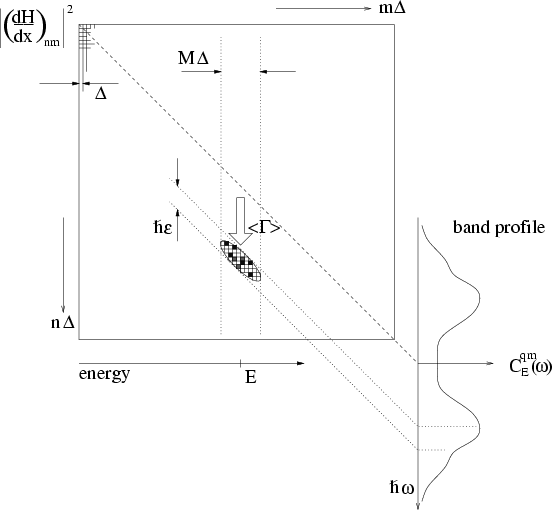
The average transition rate
is given by the local mean value near the location
  in the matrix
(see Fig. 2.3).
This will next be formalised using the `band profile' of the matrix.
Figure:
Relation of the band profile
 to the squared matrix elements
 around
 .
The diagram of the matrix has energy units in both axes.
The local average of the transition rate
  is taken over an ellipse whose horizontal width is
an energy range
  , and whose width in the
off-diagonal direction is and energy range
 .
Both widths are
  , the mean level spacing.
The width
  is classically small.
 |


Next: Generalized force-force correlation and
Up: Review of the linear
Previous: Review of the linear
Alex Barnett
2001-10-03
![]() on which the Hamiltonian depends.
The parameter is externally controllable with any (real)
function of time
on which the Hamiltonian depends.
The parameter is externally controllable with any (real)
function of time ![]() ;
it does not have any dynamics of its own (it is not a degree of freedom).
We start by linearizing about
;
it does not have any dynamics of its own (it is not a degree of freedom).
We start by linearizing about ![]() ,
,

![]() ,
,
![$\displaystyle \frac{1}{\hbar^2} \frac{A^2}{4} \left\vert \left( \frac{\partial ...
...ega)t +
\mbox{sinc}^2 \mbox{\small$\frac{1}{2}$}(\omega_{nm} + \omega)t \right]$](img272.gif)
![]() is assumed
to be a smooth function of
is assumed
to be a smooth function of ![]() , enabling it to be taken as constant
over the width of the delta-function--
this is often true in integrable systems.
In contrast, in
a chaotic system
it takes essentially
random, uncorrelated values at each
, enabling it to be taken as constant
over the width of the delta-function--
this is often true in integrable systems.
In contrast, in
a chaotic system
it takes essentially
random, uncorrelated values at each ![]() and
and ![]() (this assumption
underlies any Random Matrix Theory[35,146]
description of chaos).
The average transition rate
is given by the local mean value near the location
(this assumption
underlies any Random Matrix Theory[35,146]
description of chaos).
The average transition rate
is given by the local mean value near the location ![]() in the matrix
(see Fig. 2.3).
This will next be formalised using the `band profile' of the matrix.
in the matrix
(see Fig. 2.3).
This will next be formalised using the `band profile' of the matrix.
