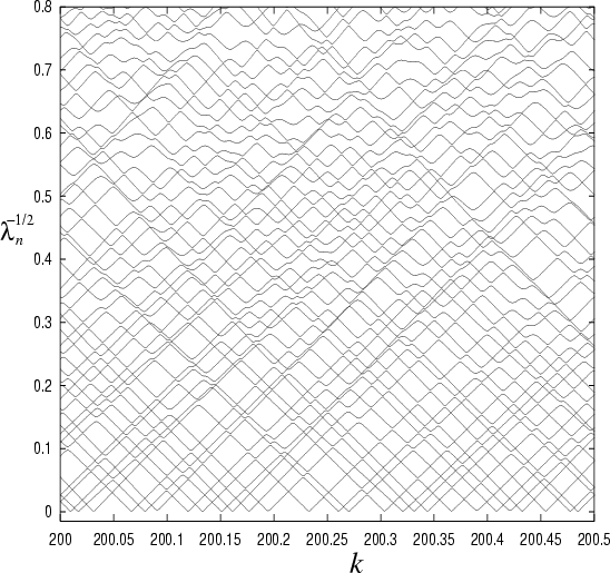
What are the prospects for a more intelligent `hunt' procedure?
It is interesting that the individual matrix elements of ![]() and
and ![]() are linear up to a
are linear up to a ![]() -scale of
-scale of
![]() , the inverse system length
(this is because the basis functions generally oscillate at a wavenumber
, the inverse system length
(this is because the basis functions generally oscillate at a wavenumber ![]() ).
This scale is
).
This scale is
![]() times larger than the average level-spacing
in
times larger than the average level-spacing
in ![]() .
This implies that information about all the tension minima in
a
.
This implies that information about all the tension minima in
a ![]() range
range
![]() might be contained in
might be contained in ![]() and
and ![]() and their
and their
![]() -derivatives
at a single
-derivatives
at a single ![]() value.
value.
To take a `toy problem' example,
imagine the values of ![]() are desired such that a parameter-dependent
order-
are desired such that a parameter-dependent
order-![]() symmetric matrix
symmetric matrix ![]() has a zero eigenvalue.
We assume linear dependence
has a zero eigenvalue.
We assume linear dependence
![]() .
The zero eigenvalue condition is written
.
The zero eigenvalue condition is written
![]() .
This is simply the generalized eigenvalue equation between
.
This is simply the generalized eigenvalue equation between ![]() and
and ![]() ,
whose once-off diagonalization predicts all
,
whose once-off diagonalization predicts all ![]() solutions of
solutions of ![]() .
This sounds promising, however the types of zero-crossings produced in
the eigenvalues of
.
This sounds promising, however the types of zero-crossings produced in
the eigenvalues of ![]() are linear (passing through zero with finite
slope, changing sign in the process). Unfortunately the methods of this
chapter require detection of eigenvalues of positive definite matrices
which reach (close to) zero in a quadratic fashion (they cannot change sign).
Therefore the above trick is no help.
are linear (passing through zero with finite
slope, changing sign in the process). Unfortunately the methods of this
chapter require detection of eigenvalues of positive definite matrices
which reach (close to) zero in a quadratic fashion (they cannot change sign).
Therefore the above trick is no help.
In fact, the above linearization of ![]() and
and ![]() is deceptive, since
their positive-definiteness cannot be maintained without considering
higher-order powers of
is deceptive, since
their positive-definiteness cannot be maintained without considering
higher-order powers of ![]() .
The positive-definite nature of
.
The positive-definite nature of ![]() and
and ![]() arises because they are the square
of other matrices (e.g.
arises because they are the square
of other matrices (e.g.
![]() , see Appendix G).
It is these other matrices whose entries can unproblematically be linearized
in
, see Appendix G).
It is these other matrices whose entries can unproblematically be linearized
in ![]() .
If we imagine again the toy problem now with
.
If we imagine again the toy problem now with
![]() and
and
![]() .
Eigenvalues of
.
Eigenvalues of ![]() are given by squares of singular values of
are given by squares of singular values of ![]() [81].
So now the problem is to predict the singular value zero-intersections
of
[81].
So now the problem is to predict the singular value zero-intersections
of ![]() (of course, this is the problem common to all Class b) methods, and
is therefore of huge interest).
Unfortunately the generalized singular value decomposition
[81] of
(of course, this is the problem common to all Class b) methods, and
is therefore of huge interest).
Unfortunately the generalized singular value decomposition
[81] of ![]() and
and ![]() does not predict these
does not predict these ![]() values.
Even though all the information about the
values.
Even though all the information about the ![]() values is contained in
values is contained in ![]() and
and
![]() , I am unaware of a suitable decomposition which returns these values.
It is an area for future research, and would have a huge impact on the large
physics and engineering community currently using Class b) methods.
, I am unaware of a suitable decomposition which returns these values.
It is an area for future research, and would have a huge impact on the large
physics and engineering community currently using Class b) methods.
One untested idea on this front is the presentation of the toy problem
as
![]() , where
, where
![]() and
and
![]() .
It is possible to convert this nonlinear eigenvalue problem into a linear
one of order
.
It is possible to convert this nonlinear eigenvalue problem into a linear
one of order ![]() (see e.g. [161]),
(see e.g. [161]),
 |