The cavity system

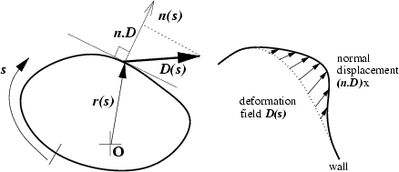
Figure: Left: Coordinates and local outward normal direction. The boundary deformation function is $D{({\mathbf s})}\equiv {\mathbf n}\cdot{\mathbf D}$. Right: Action of deformation field on wall for finite parameter $x$ (the undeformed wall for $x=0$ is shown by a dotted line).

Consider a single particle whose canonical coordinates are $({\mathbf r},{\mathbf p})$ moving inside a cavity of $d$ . The Hamiltonian is

$${\mathcal{H}}({\mathbf r},{\mathbf p};x) = {\mathbf p}^2/2m + U( {\mathbf r} - x{\mathbf D}({\mathbf r}) )$$ (3.1)

where $U({\mathbf r})$ is the confining potential. I have introduced a (unitless) deformation `field' ${\mathbf D}({\mathbf r})$, so the effect of changing the parameter $x$ is to distort the potential in space. We assume that $U({\mathbf r})=0$ inside the cavity. Outside the cavity the potential $U({\mathbf r})$ becomes very large. To be specific, one may assume that the walls exert a normal force $f$, and we take the hard wall limit $f \rightarrow \infty$. With the above assumptions about $U({\mathbf r})$ it is clear that the deformation is completely specified by the scalar boundary deformation function $D({\mathbf s}) \equiv \hat{{\mathbf n}}({\mathbf s})\cdot{\mathbf D}({\mathbf s})$, where $\hat{{\mathbf n}}({\mathbf s})$ is an outwards unit normal vector at the boundary point ${\mathbf s}$. This is shown in Fig. 3.1. The surface area of the cavity is ${\mathsf{A}}$. Its volume is ${\mathsf{V}}$, which is related to its typical length ${\mathsf{L}}$ by ${\mathsf{V}}= {\mathsf{L}}^d$. Quantum-mechanically, a second length scale $\lambda_{{\mbox{\tiny B}}}\equiv 2\pi/k$ appears, where $k$ is the wavenumber. The other parameters $v$ (particle velocity) and $m$ (particle mass), as well as $\hbar$, could be scaled away with the appropriate choice of units (this will only be done in numerical tests where we set $m=v=\hbar=1$). The energy is $E=\mbox{\small$\frac{1}{2}$}mv^2$. Sometimes I will use $v_{{\mbox{\tiny E}}}$ to denote $v$ corresponding to energy $E$. Upon quantization the eigenenergies, which in general are $x$-dependent, are $E_n=(\hbar k_n)^2/2m$.

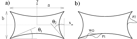
My numerical calculations of the band profile in this and the following chapter, unless otherwise stated, will refer to the two-dimensional (2D) cavity illustrated in Fig. 3.2, which we call the generalized Sinai billiard. The shape has been chosen because it has `hard chaos': no mixed phase space, and absence of any marginally-stable orbits (see Section 3.4). In Fig. 3.2b we show three example deformations of this billiard.

The band profile calculations will generally be done classically (Appendix B), since this is easier by far than the quantum calculation (Appendix C). The two have been demonstrated equivalent in Section 2.3. In Section 3.3.2 I will verify this equivalence for special deformations.

Figure 3.2: a) The example (undeformed) cavity used for numerical studies (unless otherwise stated): a generalized two-dimensional Sinai billiard formed from concave arcs of circles with two different radii. Typical parameters used are $a{=}2$, $b{=}1$, $\theta_1{=}0.2$, $\theta_2{=}0.5$, for which the average collision rate with the wall is $(1/\tau_{{\mbox{\tiny bl}}}) \approx 0.63$. b) Sketches of the effect of three of the deformation types on the perimeter (here we have chosen three localized deformations; see Tables 3.1 and 3.2 for functional forms of all deformations used). The deformations are shown exaggerated in strength.