Correction of the eigenwavenumbers

In Fig. 6.4 (bottom) the consistent curvature in the predicted shifts $\delta$ implies that higher-order effects could be important in predicting the $k_\mu$ values. There are many levels of higher-order correction possible once the basic diagonalization of (6.25) has been performed: 1) identification of the higher-order diagonal terms in $\tilde{F}$ and $d\tilde{F}/dk$ for an average state, then correcting all the $k_\mu$ according to the same resulting formula, 2) using $\partial_n \psi_\mu$ for each state on the boundary to compute a correction for each corresponding $k_\mu$, 3) using $\partial_n \psi_\mu$ for each state on the boundary and knowledge of off-diagonal terms in $\tilde{F}$ and $d\tilde{F}/dk$ to compute corrections to the eigenvectors ${\mathbf x}_\mu$ as well as the $k_\mu$. I will only report on the first of these ideas, since it is easiest to routinely implement. The other two levels of correction are areas for investigation, however it is not known whether they will prove even worthwhile (there is a trade-off betweeen correcting the results of one diagonalization and simply performing more diagonalizations). My inkling is that in practice the corrections presented here will be the only worthwhile ones.

Appendix I shows that the expansion of the diagonal of the tension matrix is

$$\tilde{F}_{\mu\mu} \ = \ 2\delta_\mu^2 - 2 \frac{\delta_\mu... ...5 {\mathsf{L}}^2}{k_\mu}) + O(\delta^6 {\mathsf{L}}^4) \cdots$$ (6.27)

where the coefficient $C_4$ is the sum of many complicated boundary integrals of $\partial_n \psi_\mu$, $\partial_{nt}\psi_\mu$, etc, and the local curvature $\alpha$ and its derivative. It is possible in theory to perform a random-wave estimate for these integrals to reach an expression in terms of the billiard shape. However in practice it is much easier to fit for $C_4$ by measuring the average value for a few states. For instance, in the quarter stadium of length 2 by height 1, $C_4 \approx -1.3$. However, it varies from state to state ^6.3, taking smaller values for states with higher average transverse momentum on the boundary, or for states which are scarred so as to avoid regions of high $r_n$. Note that $C_4$ has units of length squared, so that if the billiard changes size, then $C_4$ will need to be scaled accordingly.

The generalized eigenvalue is $\lambda_\mu = (d\tilde{F}_{\mu\mu}/dk)/\tilde{F}_{\mu\mu}$ which can be found from (6.27). Inversion of the series expansion is needed to get the series for our estimate for $\delta _\mu$, giving

$$k_\mu \ \equiv \ k - \delta_\mu \ = \ k - \frac{2}{\lambda_... ...c{4 C_4}{\lambda_\mu^3} + O(\frac{1}{\lambda_\mu^4}) \cdots ,$$ (6.28)

where corrections of $O(\delta_\mu/k)$ have been ignored. This is our improved version of (6.26). In tests, use of this formula had little effect on the $N/100$ most accurate states, but the resulting wavenumber shift reduced the tension of the remainder of the useful states by a factor of $\approx 8$ (see Fig. 6.9). Also, the $O(\lambda_\mu^{-2})$ term had very little effect (much less than the $O(\lambda_\mu^{-3})$) because of the $1/k$ factor. The utility of higher-order expansion is minimal (the next significant, the sixth-order, has little effect).

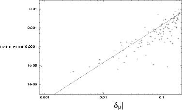
Figure 6.8: Automatic normalization of states returned by the scaling method at $k\approx 10^3$, using (6.29). The error from 1 is shown. The growth of random norm errors roughly follows a second power law (shown by the staight line).