Point contact coupled to a resonator

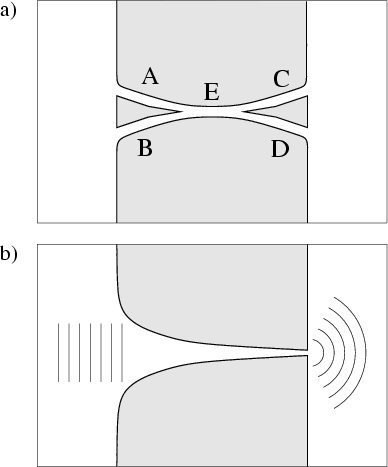
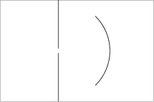
Fig. 7.3 illustrates a QPC-plus-reflector system whose conductance has been experimentally measured [112]. The circular arc reflector and the vertical wall together form a cavity which can support long-lived resonances; the energy of these resonances can be swept by sweeping the reflector gate voltage. The classical condition for stability of the cavity modes is that the arc center must lie at, or to the left of, the wall ($x{=}0$) [112]. The cavity modes are coupled to the left terminal via the QPC, and to the right terminal via leakage of the modes out through the cavity top and bottom. The system is interesting because it is `open' in the sense that it has no Coulomb blockade [20], but `closed' in the sense that the dwell time is much greater than the ballistic time (the resonances are long-lived). It has also been studied recently in our laboratory using microwave measurements [94,93,95].

The actual potential in a mesoscopic experiment differs from the illustration: it has soft walls (on the scale $1/k_{{\mbox{\tiny F}}}$), it may have deviations from the circle due to lithographic error, and it has modulations of the background potential due to elastic disorder [112]. However, we will not be interested in details of the resonator on the right-hand side. Rather, we will adopt the view of a 2D scattering-theorist `looking' from the left-hand side. In this section we discuss the maximum conductance of this system, when the `bare' QPC (i.e. without the reflector) is in the tunneling regime (conductance $\ll 2e^2/h$).

Figure 7.3: A tunneling-regime QPC combined with a nearby circular reflector, forming a stable resonant cavity open at the sides.

We use the slit model from the previous section to model the QPC. This simplifies the treatment of the left-hand side scattering problem, and we do not believe it alters the basic conclusion. As before, we consider the incident plus reflected wave Eq.(7.1) when the QPC is closed to be the `unscattered' wave. This we expand in Bessel functions,

$$\psi_{{\mbox{\tiny0}}}{({\mathbf r})} = e^{i(k_{x} x + k_{y} y)} - e^{i(-k_{x} x + k_{y} y)}$$

$$= -4 i J_{1}(kr)\cos(\theta)\cos(\phi) + \mbox{\rm higher order terms}.$$ (7.20)

The first term in the expansion is the incoming plus outgoing p-wave, which in the tunneling limit, will dominate in our consideration of the absorption (as shown in Appendix K).

Now we open the slit, and replace $2 J_{1} (kr)$ in the above by $H_1^{(2)}(kr) + e^{2i\delta}\, H_{1}^{(1)}(kr)$, where $\delta$ follows the usual definition of partial-wave phase shift [128]. The closed slit corresponds to $\delta = 0$. An open slit leading into a closed resonator (imagine extending the arc in Fig. 7.3 to seal off the entire right side), in the case of infinite dephasing length, corresponds to $\delta =$ real, and would appear from the left side as an elastic dipole scatterer. An open slit with an open resonator corresponds to complex $\delta$ with positive imaginary part, and would appear as a general inelastic dipole scatterer. Therefore transmission though the QPC appears, to an observer on the left side, to be absorption of incident waves. $\sigma_{{\mbox{\tiny T}}}$ is interpreted as an `inelastic' cross section (since exiting the right-hand terminal is equivalent to leaving in a new channel), and $\sigma_{{\mbox{\tiny R}}}$ as an `elastic' one. $\sigma_{{\mbox{\tiny T}}}(k,\phi)$ can be found from integrating the net incoming flux [as in Eq.(7.5)] of the total wavefunction on the left side. Substitution into (7.4) then gives $\sigma_{{\mbox{\tiny T}}}(k,\phi) = \frac{4}{k} (1 - \vert e^{2i\delta}\vert^2) \cos^2(\phi)$ . For $\delta \rightarrow i \infty$ the maximal cross section is reached,

$$\sigma_{{\mbox{\tiny T,max}}}(k,\phi) \; = \; \frac{4}{k} \cos^2(\phi) ,$$ (7.21)

which gives effective classical area $a_{{\mbox{\tiny eff}}}= \lambda_{{\mbox{\tiny F}}}/2$. This is analogous to the fact that in 3D the effective area of an arbitrarily-small electromagnetic dipole aerial can be of order $\lambda^2$ [105]. To an observer on the left side who was able to `see' the electron waves living in the energy range $e \, \delta V$ responsible for conductance, the QPC would stand out as a `black dot' of size $\sim \lambda_{{\mbox{\tiny F}}}$ against the surrounding uniform `grey' thermal luminosity reflected in the vertical wall mirror.

The associated maximum conductance is found easily using (7.21) and (7.1) to be

$$G_{{\mbox{\tiny max}}} \; = \; \frac{2e^2}{\hbar},$$ (7.22)

the universal quantum of conductance (for 2 spin channels), independent of the size of the QPC hole, even for an arbitrarily small hole. This universal resonant-tunelling maximum conductance was first found numerically [205,110] (also see [20]); however our system differs from those of Refs. [205,110] because the resonance does not involve transmission though an isolated (zero-dimensional) quantum dot. The dramatic increase over the bare QPC conductance Eq.(7.16) runs counter to the naive classical expectation, namely that the reflector would decrease the left-to-right flow of electrons because it sends back into the QPC particles which would otherwise exit to the right.

How do we know that it is possible to build a resonant geometry which corresponds to $\delta \rightarrow i \infty$? The reflector can be described by $r$, the amplitude with which it returns an outgoing p-wave back to the QPC as an incoming p-wave. If $\vert r\vert^2 = 1 - \vert t_{11}\vert^2$, where the p-wave transmission of the QPC is $t_{11}$ [e.g. see Eq.(7.17)], then the p-wave channel becomes a 1D Fabry-Perot resonator with mirrors of matched reflectivity. Sweeping the round-trip phase then produces peaks of complete transmission (corresponding to complete p-wave absorption on the left side). The ratio of peak separation to peak width is the quality factor $Q \sim 1/\vert t_{11}\vert^2$. Such peaks, with heights much greater than the bare tunneling QPC conductance, were observed in the experiments of Katine et al.[112]. However, Eq.(7.22) has not yet been tested quantitatively because of the difficulty of matching the Fabry-Perot reflectivities in a real 2DEG experiment. Note that the maximum conductance (7.22) also follows immediately from the Landauer formula, when we realize that there can be complete transmission of the incoming $l{=}1$ channel state (in Section 7.2).

An interesting possibility arises when we realize (Appendix K) that higher $l$ channels are still slightly transmitted by the bare QPC, when $ka \ll 1$, even though they are increasingly evanescent. If the resonator has a high enough reflectivity for these modes, then additional Fabry-Perot conductance peaks will be produced [205,38]. The peaks may be extremely narrow, but can carry a full quantum of conductance because they can transmit another incoming $l$ channel. By careful arrangement of the cavity, one or more of these peaks could be brought into conjunction with an already-existing $l{=}1$ peak at the Fermi energy. (For instance, the $l{=}1$ and $l{=}2$ resonances are in different symmetry classes in Fig. 7.3 so there can be an exact level crossing). Therefore, we have the surprising result that, in theory, a conductance of $(2e^2/h) n$ can pass through an arbitrarily small QPC hole if $n$ resonances (from $n$ different channels) coincide at the Fermi energy. However, due to their extremely small width, such large conductance peaks are unlikely to be observable in a real mesoscopic tunneling QPC due to finite dephasing length and finite-temperature smearing [20].

Finally, we should not overlook the fact that our expressions for partial cross sections are a factor of 4 greater than those conventionally arising in 2D scattering theory from a radial potential [128,132,3,43], because we are measuring cross section on the reflective boundary of a semi-infinite half plane. For instance, the maximum inelastic partial cross section for a single channel in free space is $\sigma_r = 1/k$ [128,132,3,43], compared to our maximum `inelastic' cross section per channel Eq.(7.21). Similarly, the maximum elastic result in free space is $\sigma_e = 4/k$, compared to our maximum (normal-incidence) `elastic' cross section per channel $\sigma_{{\mbox{\tiny R,max}}} = 16/k$. This latter case occurs when $\delta = (\mbox{integer} + \mbox{\small$\frac{1}{2}$}) \pi$.

Figure 7.4: a) An attempt to increase conductance through a single channel by multiple connections feeding from the reservoirs. All channels are single-mode and sufficiently long that the evanescent tunneling of higher modes is negligible. b) An illustrative hard-walled exponential horn system which has differing acceptance angles on each side: very narrow on the left, and very wide on the right. Such a mesoscopic 2DEG system would exhibit symmetric conductance, however, in an atom beam context the conductance can become unsymmetric.