Given the isotropic quadratic dispersion relation corresponding
to (5.2), we can choose energy units such that
![]() .
If the dispersion relation is not isotropic, it can be made so by
a re-parametrization of
.
If the dispersion relation is not isotropic, it can be made so by
a re-parametrization of ![]() .
However, note that
.
However, note that ![]() will not play any further role.
The numerical methods described in this thesis are
really about finding the eigenwavenumbers
will not play any further role.
The numerical methods described in this thesis are
really about finding the eigenwavenumbers ![]() .
Therefore the methods are entirely applicable to any other Helmholtz
eigenproblem regardless of the dispersion relation, or indeed the existence
of an `energy' (for instance
.
Therefore the methods are entirely applicable to any other Helmholtz
eigenproblem regardless of the dispersion relation, or indeed the existence
of an `energy' (for instance ![]() is physically irrelevant in acoustic problems).
The only requirement is that the wavenumber be constant
(and isotropic) in the interior.
is physically irrelevant in acoustic problems).
The only requirement is that the wavenumber be constant
(and isotropic) in the interior.
The billiard has ![]() -dimensional `volume'
-dimensional `volume' ![]() and
and ![]() dimensional
`surface area'
dimensional
`surface area' ![]() , giving a typical length scale
, giving a typical length scale
![]() .
Our eigenproblem can be written
.
Our eigenproblem can be written
The BCs have been incorporated as (5.6)
rather than the linear condition (5.3)
because satisfaction of the BCs by a wavefunction ![]() is then
revealed by a single number
is then
revealed by a single number ![]() .
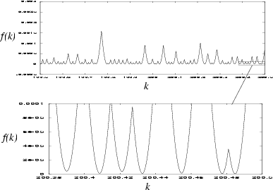
This number measures the 2-norm of some error function,
and is therefore a non-negative quantity.
The error function (e.g. (5.3)) gives the amount
by which the desired BCs fail to be obeyed.
Heller[91] named
.
This number measures the 2-norm of some error function,
and is therefore a non-negative quantity.
The error function (e.g. (5.3)) gives the amount
by which the desired BCs fail to be obeyed.
Heller[91] named ![]() `tension', and I shall follow suit.
The definition of
`tension', and I shall follow suit.
The definition of ![]() is
is
Without a further condition, (5.5) and (5.6) admit the
useless solution,
![]() for all
for all ![]() .
Therefore the quadratic functional
.
Therefore the quadratic functional
The solution
![]() is now completely determined, when
is now completely determined, when ![]() reaches one
of the eigenwavenumbers
reaches one
of the eigenwavenumbers ![]() .
For other
.
For other ![]() , no solution exists.
Therefore in order to be able to define a `best' solution for any
given guess
at
, no solution exists.
Therefore in order to be able to define a `best' solution for any
given guess
at ![]() , one of the conditions needs to be relaxed.
The condition (5.6) will be replaced by the minimization
, one of the conditions needs to be relaxed.
The condition (5.6) will be replaced by the minimization
 |